## Automated Landmarking of the Human Skull

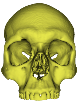
Project description: I was assigned a project to landmark human skulls for an intro to geomorphometrics (GM) class. The assignment was based on manual plotting of landmarks using MeshLab, an outdated 3D mesh analysis software. In the spirit of modernization and leveraging novel methodologies I turned to 3D Slicer, a modern medical analysis software that contains an extension, SlicerMorph, designed to streamline the GM process. What follows is my first steps in attempting to fully automate the landmarking process of the human viscerocranium for this class project as well as the gathering of novel data to test the general applicaiton of these methods.

Note: All skulls imaged here are not archaeological artefacts. The images here are manipulated stand ins created with the free 3D skull model available here.

Semi Automatic vs Automatic Processes.

For my class project I was given 11 skulls. 5 male, 5 female, and 1 NA or not assigned. The goal was to attempt to determine the sex of the NA skull and assess researcher error. In MeshLab you would need to manually place landmarks across each skull. This is slow for large amounts of landmarks. Additionally, MeshLab exports files in a .pp format which seems to be an HTML style data storage method. This reduces cross platform usability e.g. importation into R for further analysis.

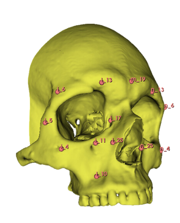
As this process of manual landmark placement is arduous and slow but widely used by arcaheologists, I decided that the first automated landmarking method should resemble the original process, just make it much more efficient. My reasoning here is that archaeologists can be incredibly slow to adapt to new technology, perhaps if it resembles a process which they already follow then they would be less reticent to try this new process. As such, the first step of what I call the semi automatic method required the manual creation of a set of landmark points across traditional osteological points of interest on the skull. I used this paper by Toneva et al. as a basis for choosing the viscerocranium to determine sex as well as to have a systematic landmarking system. I chose a number of landmarks used in their study and manually recreated their position resulting in the following figure:

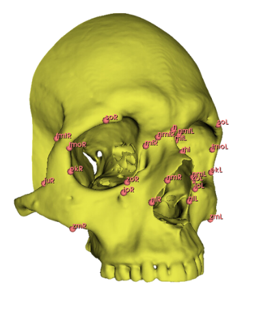
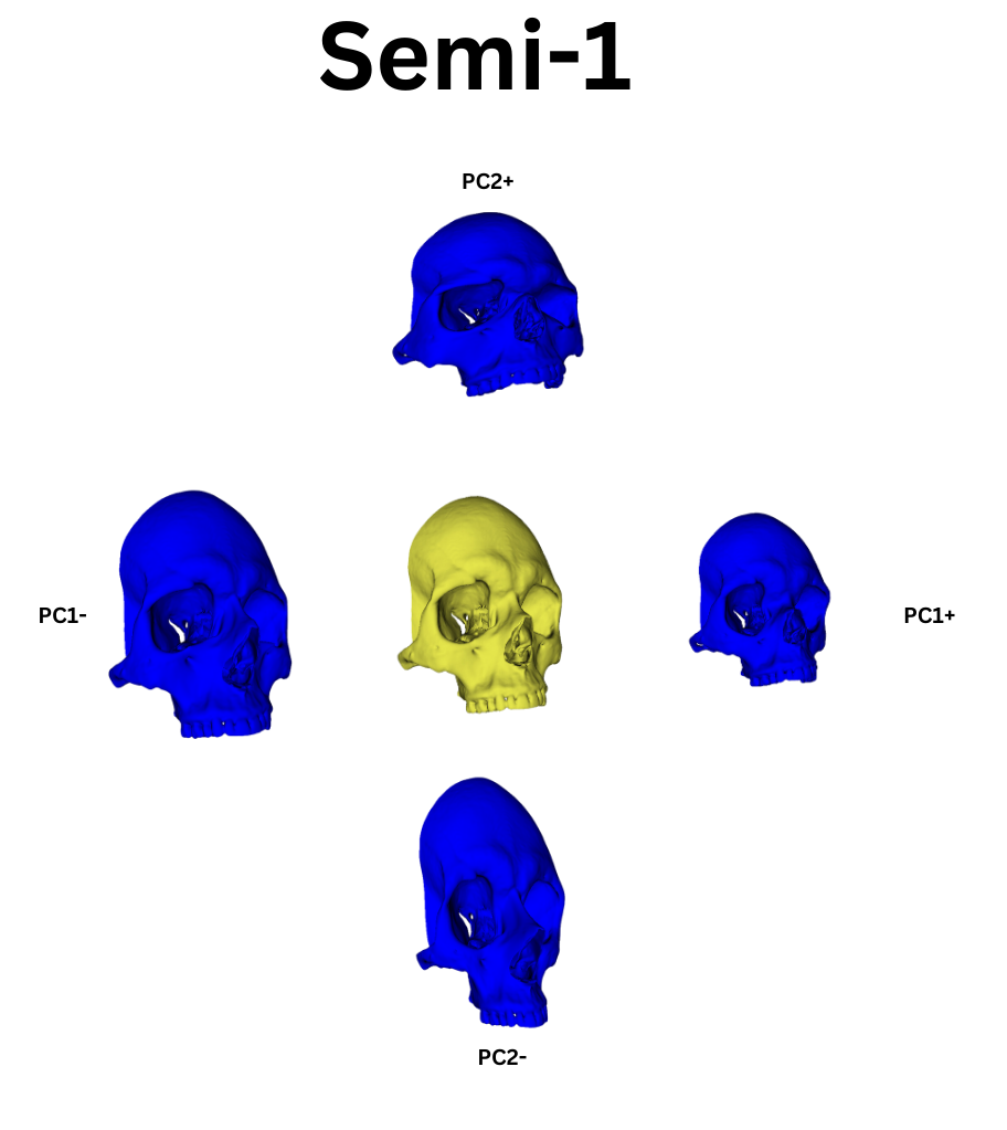
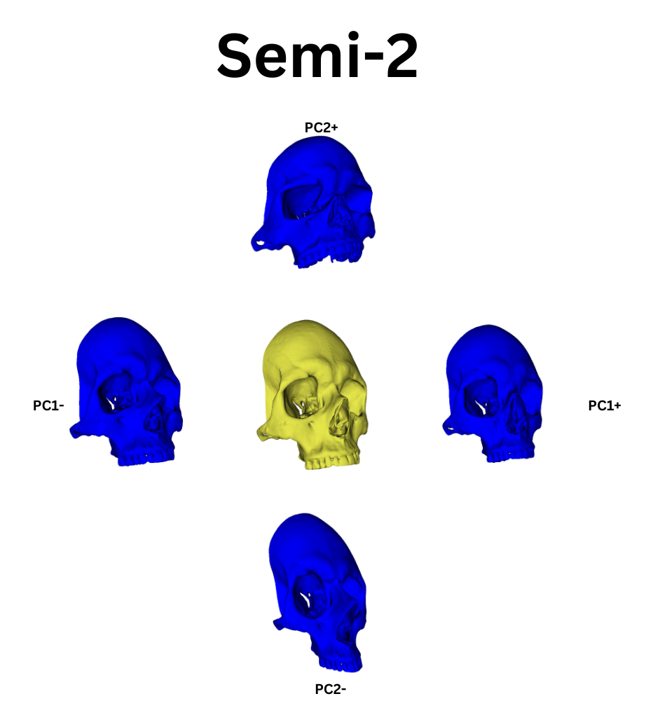
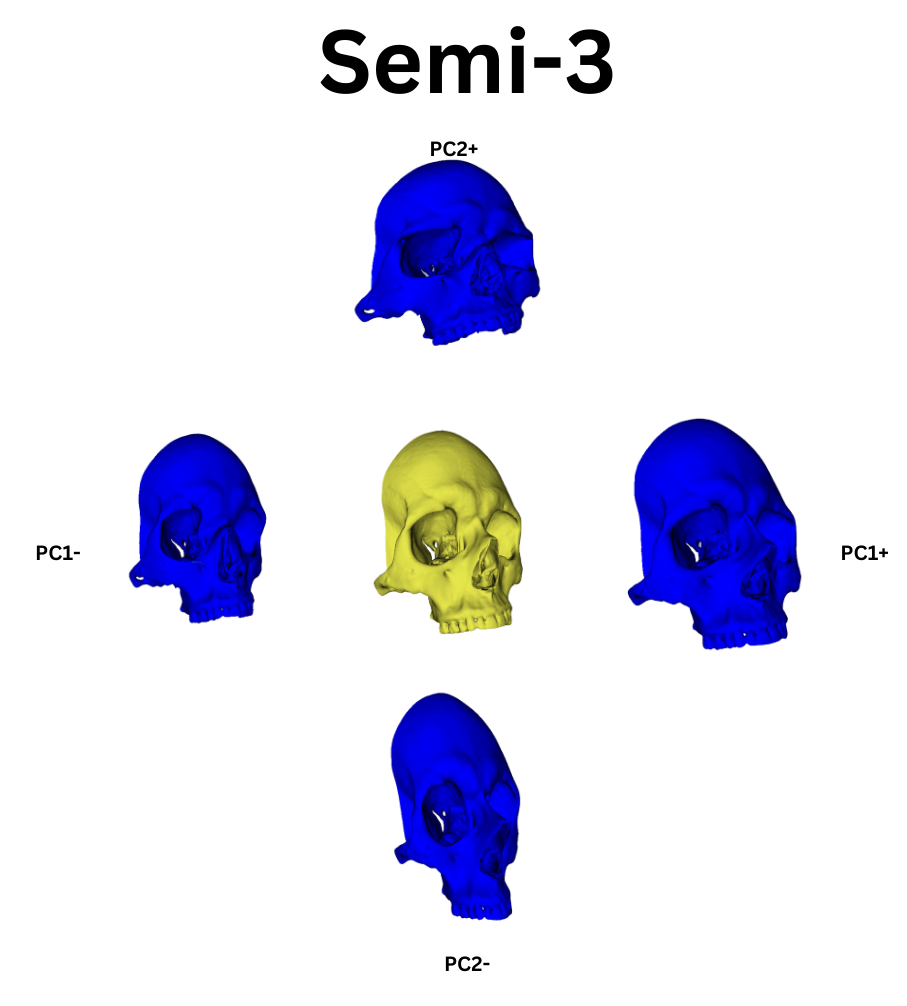
From this point, I leveraged a module named Automated Landmarking through Pointcloud Alignment and Correspondence Analysis or ALPACA. This module is absolutely amazing. It can take in a single set of points and a corresponding model and it will attempt to place a similar set of points across other selected models. Additionally, if your data set is large enough, ALPACA can batch process a few input models and sets of points to increase its accuracy placing landmarks across yoru other data. For my purposes, I input a single model and set of points to ALPACA then went over the autogenerated points and hand corrected any errors. I repeated this process twice over the whole data set to give me three separate sets of manually corrected autogenerated points. This would act as an analogue to researcher error measurements by comparing the accuracy of my hand curation of the auto generated points by measuring the variation in the placement of the landmarks across the three data sets. In additon to simply generating the points, I ran the GPA and PCA over them which allowed me to warp the average shape of the skull via the PC eigenvectors. The figures below show the average skull shape for each ALPACA data set as well as their PC1/2 warps along each axis:

To extend the idea of automation further, I used another tool, PseudoLMGenerator (PLMG), which can automatically place landmark points across any surface. As the semi auto method was tested on the viscerocranium, when I used PLMG to generate landmarks I deleted every landmark outside this region of interest. The issue with PLMG is that it will create a bespoke landmark set for each input mesh. As such, comparing landmarks between skulls would be impossible. As such, I chose to use PLMG on one skull and then put its output into ALPACA. In the spirit of complete automation I decided to not hand curate the ALPACA points. This had two benefits. The first was that both ALPACA and PLMG have various hyper parameters that can be adjusted to increase their accuracy or change their behavior. While I wanted to investigate these, to do this programatically I would have needed to learn how 3D slicer constructs its data structures in order to extract the relevant data. While not too difficult, I am currently pressed for time with PhD applications and graduation bureaurocracy. This will have to be shelved until I get enough free time to revisit the process. Regardless, my metric of comparason between this automatic method and the previous semi auto method would be to observe if their landmark points produced similar clustering behavior after being run through a Generalized Procrustes Analysis (GPA) and Principle Component Analysis (PCA).

GPA -> PCA Results

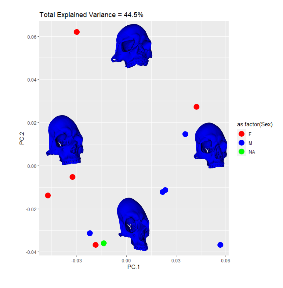
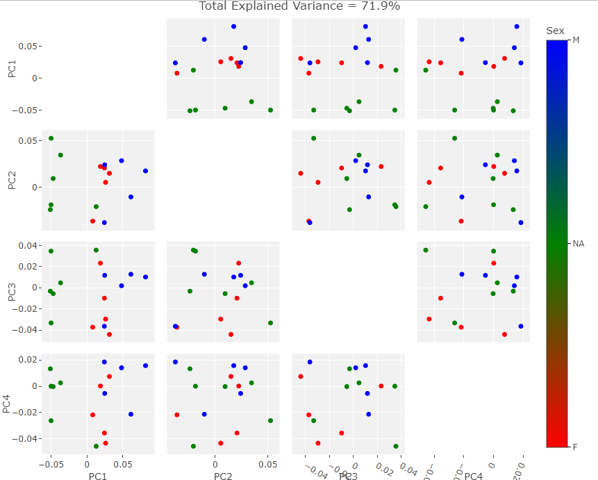
The SlicerMorph package contatins a GPA tool. All you need do is point it to the directory input data landmarks and it will run the GPA as well as a PCA. The results from the semi and fully automatic methods were subjected to this process. I exported the results to R for plotting. The first comparison in behavior between the two methods can be seen in the clustering along the first four PC components. Males are blue, Females are Red, and the NA point is in Green. I’ve placed black lines across the 1st PC component comparasons in order to highlight the binary clustering structure.

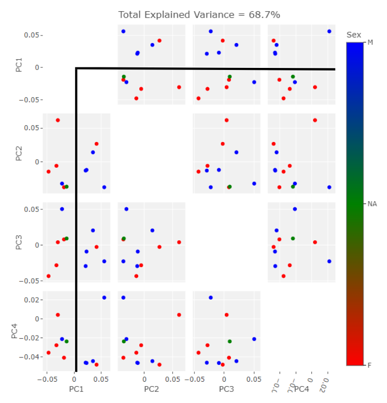
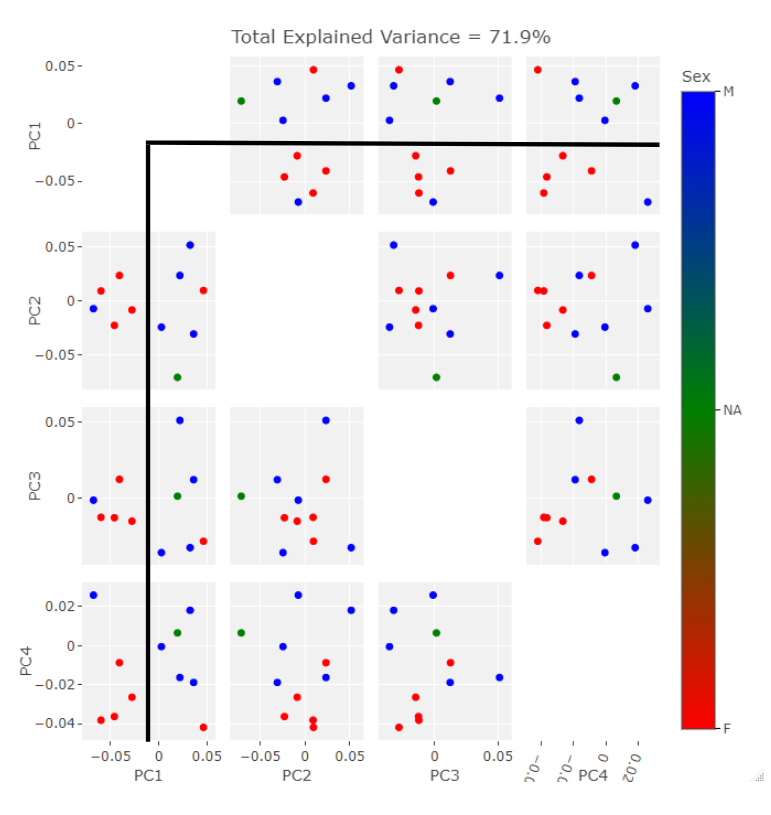
The clusters in both cases are largely segregated by Sex. However, there is one male point in the female group and one female point in the male group. This is a relatively small data set so perhaps these outliers would be less suprising in their reciprocity with more input data. The major difference observable here is the NA point in the semi auto data is in the mostly female group while it is in the mostly male group in the auto data.

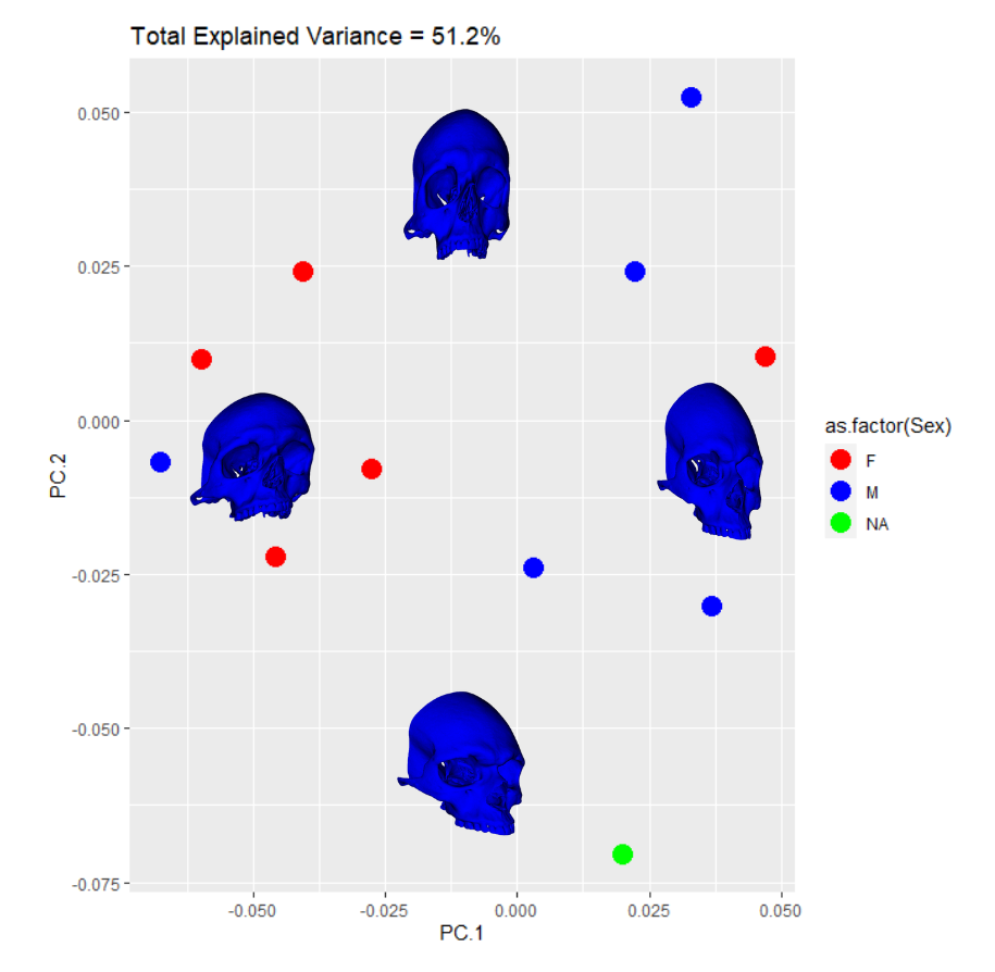
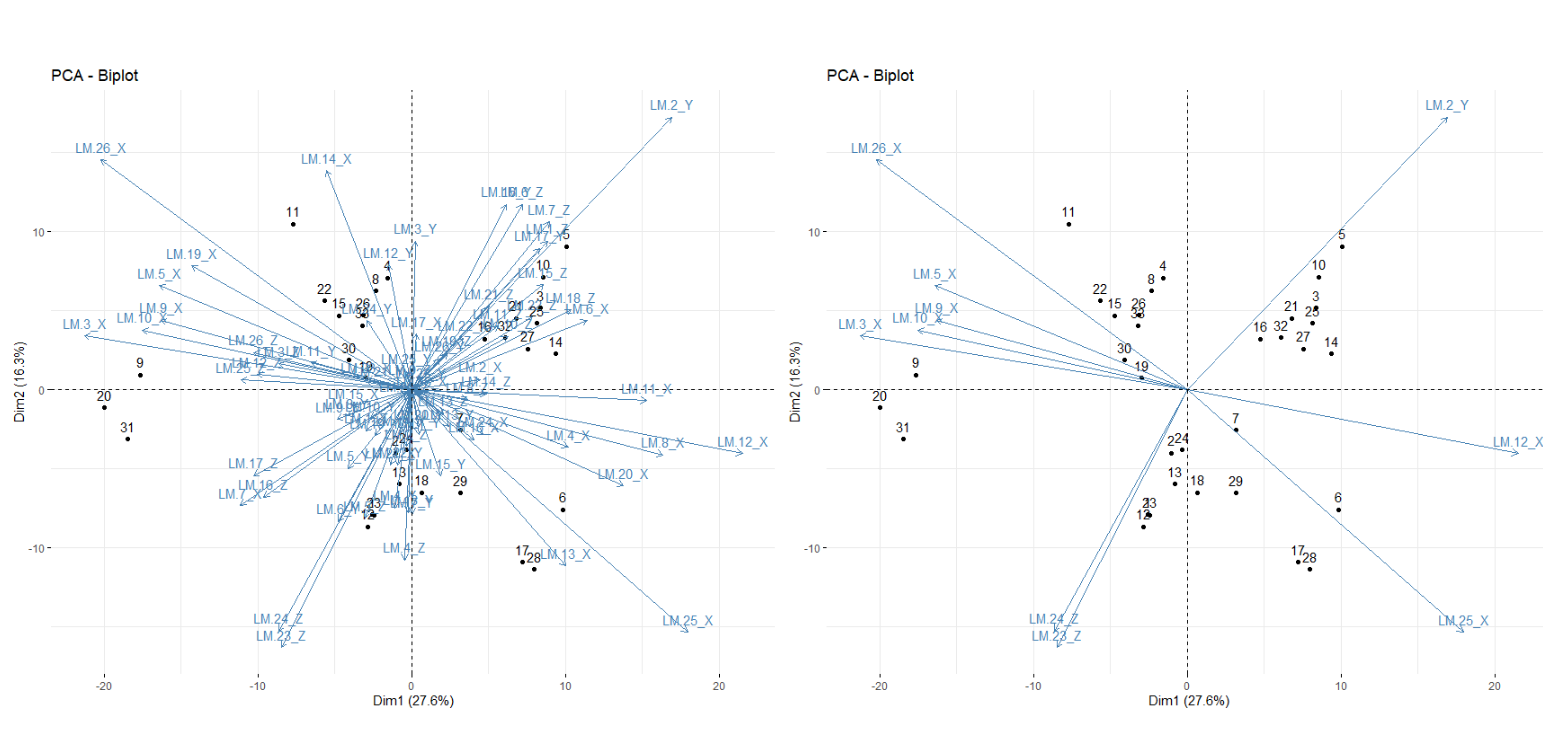
A more interesting way to display this data can be created when you add the PC warps to singular biplots. This can be useful when you have significant variance captured by the first two PC components or you just want to illustrate to your audience exactly what the PC vectors represent in real space while also showing the behavior of your data in PC space:

LDA Confirmation

To confirm these visual results mathematically I used the klaR package in R to run a linear discriminate analysis across PC space for each of the 3 semi auto as well as the automatic data sets. For each data set I first generated comparisons between each binary pair of PC components which resulted in the messy plot below:

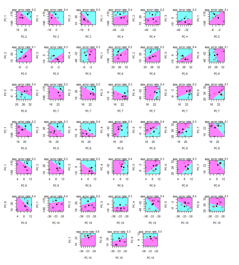
This plot is nasty to look at but it gives you an error score for classification across each pair. In the above example the pair with the lowest error score is P2 vs PC5. The second ALPACA Run had the lowest biplot discrimination error rate along PC1 vs PC10, which is shown below with the NA point added in green:

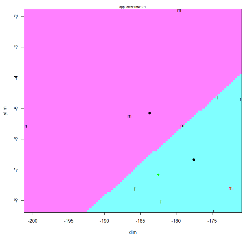
It is kind of insane to reach into the 10th PC dimension to look for meaningful clustering patterns as PC10 represents such a small amount of variation. So while we can generate plots like these for each data set and we can hope that maximal divisibility will occur across PC1 and PC2 to better justify our results this is not a scientific approach. Rather, I used LDA across every PC dimension to find the multivariate linear model that best described the separation between male and female points. Running this model over NA’s PC data gives us the following posterior results:

Run	Posterior Male	Posterior Female
Semi-Auto 1	0.59	0.41
Semi-Auto 2	0.48	0.52
Semi-Auto 3	0.52	0.47
Automatic	0.47	0.53

Table: Semi Auto and Automatic LDA Posterior Probabilities

These results show that the results of our previous visual inspection were correct in that the semi auto method generally thinks the NA point is a female and the auto method results point to NA being a male. However, in general, the posterior probabilities were extremely close for the categorization of male or female. Perhaps the most firm conclusion we can reach in regards to the sex of the NA individual is that it is indeterminate.

Visualizing Measurement Error in Semi Auto Runs

The differing results of LDA across the semi auto runs is due to the variation in the placement of the landmarks during the hand curation process. We can simplistically visualize this error by looking at a traditional PC1 vs PC2 biplot. This is done below and the centroid of the three point landmark clusters is shown to better see the distance between each point:

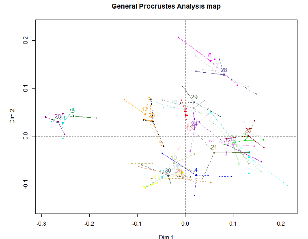
I find this plot unintuitive and kind of ugly. SlicerMorph allows you to visualize the variation in measurement between the different sets of points it uses for a GPA. As such I took the average landmark shape from each ALPACA run, ran a GPA over them, and visualized the variation in measurement between the averages:

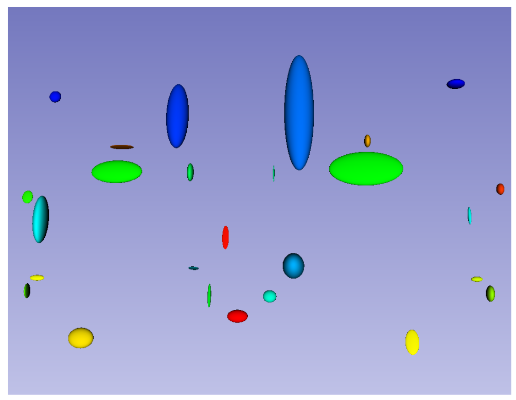
This plot is rotatable in 3D space and you can focus in on areas of interest. In this case each ellipse shows the magnitude and direction of variation for each point. This is a quick visual way to see what data points have the most error, which might need remeasuring, and which are the most accurate.

Novel Data Generation and Analysis

I used an Artec Space Spider Blue-Light 3D Scanner, to create 6 new models for processing. For my own practice I scanned the entirety of the skulls but pre-processed this data in 3D scanner and cut it down to match the sections of skulls used up to this point.

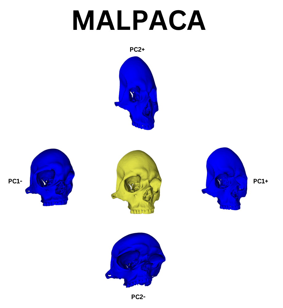
ALPACA can accept multiple input templates to create a more accurate placement of autogenerated landmarks on new data. When used in this way the process is referred to as MALPACA. I used a k-means selection algorithm packaged into slicer morph to find the 3 most representative models from the example data set. I took the hand curated ALPACA results for these and fed them into MALPACA to automatically generate landmark points to the new scans. This process is computationally intensive and would be greatly aided by a newer computer than mine, which is five years old and on its last legs. Creating new landmark points over a large dataset of dense models could take hours, if not days, without proper computational resources. It is a good idea to test this process on a single model as a rough test of how long you might expect MALPACA to run over your entire data set.

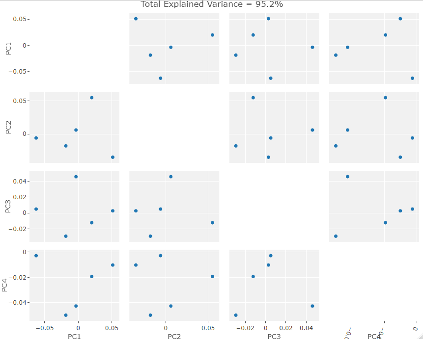
I subjected the results of the MALPACA process over the new data to the same statistical and visualization processes that were used to evaluate the example class data. These results are summarized in the figures below. As I do not know the sex of these individuals, I decided to not perform LDA but rather compare the PCA results between each set of data. The following three figures are: New Data PCA Warps; PCA, Only New Skulls; PCA, All Data (except original NA point),

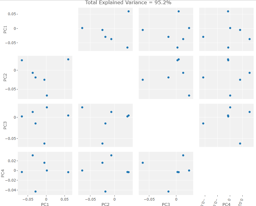
Visually the PC eigenvectors cause the average model of the new data to warp in a similar way to the semi and fully automatic output. The PCA results from the new data show a similar division in PCA scores to the example ones in that there are two distinct groups. As I chose the skulls randomly we cannot separate them into male in female groups as of yet but further archival research will hopefully unearth a previous evaluation of the skulls’ sexes. It is important to note that while these skulls do seems to exhibit the same clustering as the example data, as there is only one data point in one of the clusters. This may simply be an outlier skull. Evaluating the normality of the potential outlier with such a small sample size is statistically difficult. However, by removing that skull from the data set and rerunning the GPA/PCA we can scale the remaining points to see if they exhibit strong clustering behavior without the outlier. This is shown below:

The clustering is ambiguous at best but again this is a small sample size so statistical testing over a larger data set would definitely be beneficial. If we ignore this glaring issue then we could say that the resultant ambiguity points to the “outlier” not really being an outlier. Rather it is a singular sex divided from 5 examples of the other sex. Thus the ambiguous clustering results when it is removed makes sense as there are no longer any large sexual geometric differences between the remaining skulls i.e. they all belong to one sex.

Determining which sex these new skulls belong to may be possible by relating their clustering to that seen in the example data. If the new skulls follow the pattern of females to the left of the biplots with males to the right then we would expect these results to mean that the new skulls consist of 5 females and 1 male. However, as this is a separate population from the example data, the division between sexes for out new six skulls could be much smaller meaning that the clustering seen in the example data would not be seen with the new data. Furthermore, perhaps the cluster of 5 new data points (the ones previously assumed to be female) could all be indeterminate within their population. These issues in interpretation are to be expected over such a small data set especially when attempting to compare it to a separate population of humans.

Though, it is important to address these concerns, these issues will be put to rest once the original evaluation of these skulls’ sexes is found. Regardless of the issues outlined above, the test with new data is a success in that MALPACA was evaluated to work on the kind of skull scans generated by researchers at the University of Tübingen. Even if the interpretations above are incorrect, the process is functional. This means that this workflow can be adopted by the osteology department in order to boost efficiency and accuracy of placing landmarks on 3D scans of human skulls.

Further Considerations

From here it may be useful to see the most important vectors in PC space in order to rate the importance of individual landmarks. This could be used to reduce the size fo the landmark set or perhaps zero in on areas of maximal importance that you need to add more landmarks in. A simple example of how to visualize this data is below:

This isn’t very useful right now as each vector is split into x,y,z components from the original landmark points. We could reformat the data to be more interpretable but that is a task for another day.

A fun additional data visualization method is to use the GPA tool from SlicerMorph to create a warp sequence for your PC eigenvectors. You can then go to the Screen Capture Module and create a .gif of the warps. I even set the skull to rotate so you can see the warping over the whole model. This could be useful for data visualization in general or for researchers to get an intimate feel for exactly what the PC eigenvectors represent. You can zoom in on specific parts of the model as well to see minute changes in the structure if you so wish. The results of my first test of this system is shown below:

Conclusion

Both the semi and fully automatic methodologies listed here have the ability to save researchers extreme amounts of time compared to the normative MeshLab based process commonly used here at Tübingen. As a novice in this field, I have only begun to scratch the surface of the various tools included within 3D Slicer. I am confident that with access to more time and computing power, I could successfully automate the landmarking procedure for any arbitrarily large set of skull scans. As of now my laptop cannot efficiently engage in more advanced procedures e.g. the registration of hundreds of semi-landmarks across large data sets. However, even the basic methods I have outlined here are more than good enough to become the new standard at our institution, and I can only hope that researchers, smarter and better equipped than I, come up with an even more efficient methodology after this one. The world is changing quickly and we must change with it. The way we do archaeology need not stay static and we should have a questing mindset, always looking for the next improvement to our science.